Electronic spectroscopy of I2
The high resolution electronic absorption spectrum of I2 will be measured around 600 nm using a combination of traditional absorption. As an extension to this investigation( to be carried out later in the semester), absorption bands will be selected for excitation and the fluorescence emission will be recorded. These results will be analyzed in terms of harmonic and Morse oscillator wavefunctions.
Overall Steps
![]() Record absorption spectrum of I2
from 540 nm - 670 nm using Ocean Optics
CCD spectrometer
Record absorption spectrum of I2
from 540 nm - 670 nm using Ocean Optics
CCD spectrometer
![]() Fluorescence emission spectroscopy
using laser excitation.
Fluorescence emission spectroscopy
using laser excitation.
![]() Analysis of vibrational wavefunctions
and theoretical prediction of intensity based on Franck-Condon principle
Analysis of vibrational wavefunctions
and theoretical prediction of intensity based on Franck-Condon principle
Method I
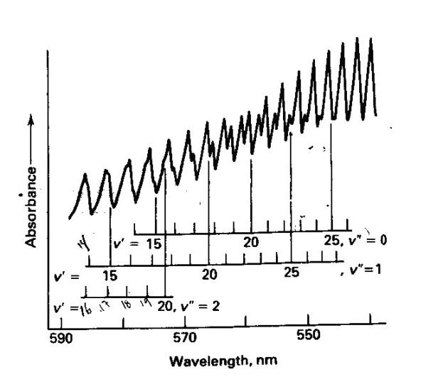
We will record the high resolution visible absorption spectrum of gaseous I2. Since we are recording the spectrum of a gas phase sample the spectrum will have sharp structure corresponding to vibrational structure superimposed on the electronic transition. In solution this structure is often not observed due to the broadening of the electronic transition due to individual molecules each have slightly different local solvent environments. The spectrum will be recorded using the Ocean Optics CCD spectrometer. The sample is contained in a sample cell with solid iodine producing sufficient vapor pressure to record an absorption spectrum. It may be necessary to supply heat to the sample to provide additional vapor pressure and a resulting increase in optical depth.
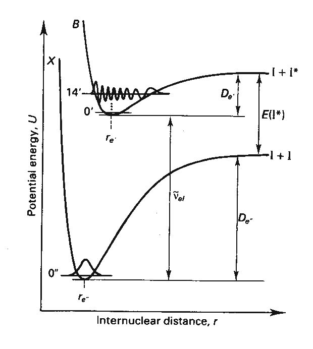
Figure 1 below shows the two
electronic states, ground and an excited state, that we will be probing in this
investigation. The electronic states
are labeled with molecular term symbols (we will cover their derivation later
in the course). The ground state has
the term: ![]() . The excited state
that we will be probing has a
. The excited state
that we will be probing has a ![]() molecular term. Each
electronic state has vibrational levels associated with it. Since there is only one vibrational mode in
I2 we only need to keep track of one quantum number.
molecular term. Each
electronic state has vibrational levels associated with it. Since there is only one vibrational mode in
I2 we only need to keep track of one quantum number.
Fluorescence emission Spectroscopy
We have measured the high-resolution electronic absorption spectrum of I2 from 560 nm - ~650 nm using traditional absorption spectroscopy. Absorption bands will be selected for excitation (as determined from our absorption spectra) and the fluorescence emission resulting from this excitation will be recorded. Later, these results will be analyzed in terms of harmonic and Morse oscillator wavefunctions.
Method II
We have recorded the high-resolution visible absorption spectrum of gaseous I2. The spectrum has relatively sharp structure corresponding to vibrational structure superimposed on the electronic transition, since we are recording the spectrum of a gas phase sample. At this point we will excite these bands with a laser and observe differences in the resulting fluorescence emission spectrum. Be sure to familiarize yourself with laser safety prior to inititing the investigation. It may be necessary to supply heat to the sample to provide additional vapor pressure and a resulting increase in optical depth.
Recall that there are two electronic
states, ground and an excited state, that we will be probing in this
investigation. The electronic states
are labeled with molecular term symbols (we will cover their derivation later
in the course). The ground state has
the term: ![]() . The excited state
that we will be probing has a
. The excited state
that we will be probing has a ![]() molecular term. Each
electronic state has vibrational levels associated with it. Since there is only one vibrational mode in
I2 we only need to keep track of one quantum number.
molecular term. Each
electronic state has vibrational levels associated with it. Since there is only one vibrational mode in
I2 we only need to keep track of one quantum number.
Electronic
Spectroscopy of Molecular Iodine
Once we identify the vibrational structure within the electronic transition from the absorption spectroscopy above we will excite a couple of these transitions using the laser to excite particular bands and record the fluorescence emission spectrum.
Prediction of the
Vibrational Structure of Iodine Electronic Spectra
After recording the absorption and emission spectra of I2, we will examine the vibrational wavefunctions of I2 using the harmonic oscillator and Morse oscillator approximations. You will analyze your experimental data in the context of these vibrational wavefunctions and Franck-Condon factors.
Vibrational
Wavefunctions
The nuclear displacement potential for diatomic molecules can be approximated by a harmonic potential, V(x)=1/2 kx^2. A better approximation, particularly at large values of the vibrational quantum number, v, is the Morse potential function, V(x)=De[Exp(-Beta*x) -1]^2, which includes a reasonable description of the dissociation of the molecule. The potential may have different forms in different electronic states due to changes in the electronic structure of the molecule leading to changes in the bonding and ultimately changes in the force constant, k, and the dissociation energy, De. We will explore vibrational wavefunctions within both the harmonic approximation and the Morse approximation. The harmonic oscillator functions have a familiar form including the Hermite polynomials. The Morse oscillator functions are more complicated but can be evaluated.
Intensity of
Electronic Transitions
The intensity of electronic transitions is determined by an electronic term, which we will assume is constant for all of our transitions, and a vibrational component which varies according to the initial and final vibrational states. A rotational term also should be included but this isn’t resolved in our spectrum so we will neglect this part. The vibrational term is known as the Franck-Condon factor and corresponds to the overlap of the final and initial vibrational wavefunctions.
Franck-Condon
Factor:  (1)
(1)
Therefore, the form of the vibrational wavefunctions in the ground, X, electronic state of I2 and the excited, B, electronic state is of interest in examining the intensity pattern observed in absorption/excitation spectra. We will examine the harmonic oscillator and Morse oscillator functions numerically in SigmaPlot. We will also numerically compute the above integral in SigmaPlot in order to predict intensity patterns. These procedures are below.
Investigation
The vibrational wavefunctions for I2 within both the Morse and harmonic oscillator approximation have been tabulated on a grid of points (r). These numerical wavefunctions are available for both the ground electronic state (X) of I2 and the B excited electronic state. These states correspond to the absorption and fluorescence emission spectra that we recorded. These functions can be imported into SigmaPlot for analysis. Generate a plot with several of these functions included.
The first step is to verify that these wavefunctions are normalized.
 (2)
(2)
Take three wavefunctions of your choice and verify that they are normalized by performing the numerical integration within SigmaPlot.
 (3)
(3)
where m is the number of points over which the wavefunction is evaluated and Dr is the spacing between points. All of the wavefunctions have the same spacing allowing this numerical procedure to apply to all of the integrals we might need to evaluate. Within SigmaPlot compute the sum of a column. How does the range on the sum compare to the range of integration? What condition is necessary for this range to be appropriate for this numeric integral?
An important property to consider is the expectation value of r as a function of electronic state, vibrational quanta, and model used to describe the potential energy function.
 (4)
(4)
Investigate the <r> for the v=0 level of each electronic state. Does the value you get make sense? Compare the <r> for the v=10, v=23, v=32 levels of the B electronic state using both the harmonic and the Morse wavefunctions. Compare and comment on these results.
Using the Franck-Condon factor expressed in equation 1 we will now investigate the relative emission intensities predicted by the Morse wavefunctions. We will only use the Morse functions because they more accurately reflect the true vibrational wavefunctions of a diatomic molecule. The particular transitions that we are interested in are between appropriate v’’ and v’ levels for the emission spectra we recorded. These v’’ and v’ values can be determined by careful examination of your spectra. For each spectrum predict the relative intensities of the first four lines using the Morse wavefunctions. Try changing the v’ value for one of your emission spectra and predict the relative intensities for three peaks. How do they compare? With one of your best two sets of predicted intensities create a simulated spectrum by using a column consisting of a sum of Gaussian functions centered at each of the emission wavenumbers. A Gaussian function centered at u has the form:
 (5)
(5)
where k is scales the amplitude of this function and thus can be used to express the relative intensity of the peaks.