Opportunities in Chemistry
A Supportive Community for Exploration
You'll find Gustie Chemistry students leading science demonstrations for elementary students for Science on Saturdays, networking and asking questions in a Chemistry seminar, or designing their own research projects. Explore the opportunities to learn outside of the classroom to enrich your college experience, gain practical skills, develop a strong professional network, and build strong relationships with other students and faculty.
Chemistry Club — This is a chance to have fun with like-minded individuals, and participate in educational initiatives and social events
Chemistry Seminar Series — Stay updated on the latest developments in chemistry, engage with off-campus experts, and deepen your understanding of the field
On-Campus Research — Participating in on-campus research projects offers a chance to engage in hands-on scientific inquiry and collaborate closely with faculty members
Off-Campus Research — Explore off-campus internships and summer research programs
Community Outreach — There are several community events to foster an interest in science among younger generations
Facilities for Learning — Nobel Hall of Science provides state-of-the-art facilities and instrumentation for learning
Explore Opportunities in Chemistry